FOSP - Study on Down sampling and Up sampling.
Study on Down sampling and Up sampling.
This post covers how to upsample and downsample data and the possible pitfalls of this process. Before we cover the technical details let us first explain what we mean by upsample and downsample and why we may need to use it.
Both these techniques relate to the rate at which data is sampled, known as the sampling rate.
We will see below that the sample rate must be carefully chosen, dependent on the content of the signal and the analysis to be performed. Imagine we have some data which has already been sampled, from a particular test or experiment and we now wish to re-analyse the data maybe using different techniques or to look for a different characteristic and we don’t have the opportunity to repeat the test. In this situation we can look at resampling techniques such as upsampling and downsampling.
Downsampling, which is also sometimes called decimation, reduces the sampling rate.
Advantages of downsampling:
- It makes the data of a more manageable size
- Reduces the dimensionality of the data thus enabling in faster processing of the data
- Reducing the storage size of the data
Upsampling, or interpolation, increases the sampling rate. Before using these techniques you will need to be aware of the following.
What is the sampling rate?
The sampling rate is the rate at which our instrumentation samples an analogue signal.
The sampling rate is very important when converting analogue signals to digital signals using an (Analogue to Digital Converter) ADC.
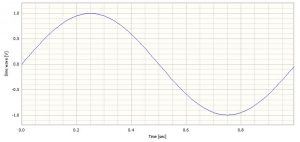
Take a simple sinewave with a frequency of 1 Hz and a duration of 1 second as shown in Figure 1. The signal has 128 samples and therefore a sampling rate of 128 samples per second. Notice that the signal ends just before 1.0 seconds. That is because our first sample is at t = 0.0 and we would actually need 129 samples to span t=0.0 to t=1.0.
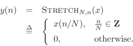
UPSAMPLING (STRETCH) OPERATOR:
.png)
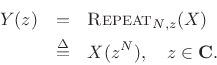
DOWNSAMPLING (DECIMATION) OPERATOR:
The symbol for downsampling by the factor . The downsampler selects every
th sample and discards the rest:

In the frequency domain, we have

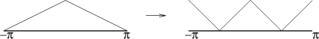
Figure: Illustration of
 )
)![\begin{eqnarray*}
Y(z) &=& \frac{1}{2}\left[X\left(W^0_2 z^{1/2}\right) + X\left(W^1_2 z^{1/2}\right)\right] \\ [5pt]
&=& \frac{1}{2}\left[X\left(e^{-j2\pi 0/2} z^{1/2}\right) + X\left(e^{-j2\pi 1/2}z^{1/2}\right)\right] \\ [5pt]
&=& \frac{1}{2}\left[X\left(z^{1/2}\right) + X\left(-z^{1/2}\right)\right] \\ [5pt]
&=& \frac{1}{2}\left[\hbox{\sc Stretch}_2(X) + \hbox{\sc Stretch}_2\left(\hbox{\sc Shift}_\pi(X)\right)\right].
\end{eqnarray*}](https://lh3.googleusercontent.com/blogger_img_proxy/AEn0k_uYydKgLqsc9BCItuT8uHFjyPSI3rifptrriSjL0UzqbRfZ-THJYnkNyHUeDURPfzWCgVc-5eVovLEyTRVo4MbW3-iRgAHqVshqdgKGZzPM4qfQz9CfxA9YQXjg=s0-d)
Examples:
Sampling Rate Increase by an Integer Factor
Increasing a sampling rate is a process of upsampling by an integer factor of L . This process is described as follows:
y(m) = { x(m/L) m = nL ,
0 otherwise, (12.9)
where n = 0, 1, 2, … , x (n ) is the sequence to be upsampled by a factor of L , and y (m ) is the upsampled sequence. As an example, suppose that the data sequence is given as follows:
x (n ):8 8 4 –5 –6 …
After upsampling the data sequence x (n ) by a factor of 3 (adding L – 1 zeros for each sample), we have the upsampled data sequence w (m ) as:
w (m ): 8 0 0 8 0 0 4 0 0 –5 0 0 –6 0 0 …
The next step is to smooth the upsampled data sequence via an interpolation filter. The process is illustrated in Figure 12-5a.

Figure . Block diagram for the upsampling process with L = 3.
fsL = Lf s . (12.10)
This indicates that after upsampling, the spectral replicas originally centered at f s , 2f s , … are included in the frequency range from 0 Hz to the new Nyquist limit Lf s =2 Hz, as shown in Figure 12-5b. To remove those included spectral replicas, an interpolation filter with a stop frequency edge of f s =2 in Hz must be attached, and the normalized stop frequency edge is given by
Ωstop = 2π (f s /2) × (T /L ) = π/L radians. (12.11)

Figure. Spectra before and after upsampling.
To verify the upsampling principle, we generate the signal x (n ) with 1 kHz and 2.5 kHz as follows:
x (n ) = 5 sin ((2π × 1000n )/8000) + cos ((2π × 2500n )/8000),
with a sampling rate of f s = 8,000 Hz. The spectrum of x (n ) is plotted in Figure 12-6. Now we upsample x (n ) by a factor of 3, that is, L = 3. We know that the sampling rate is increased to be 3 × 8000 = 24,000 Hz. Hence, without using the interpolation filter, the spectrum would contain the image frequencies originally centered at the multiple frequencies of 8 kHz. The top plot in Figure 12-6 shows the spectrum for the sequence after upsampling and before applying the interpolation filter.

Figure. (Top) The spectrum after upsampling and before applying the interpolationfilter(bottom) the spectrum after applying the interpolation filter.
Ωc = 2π × 3250 × (1/24000) = 0.2708π.
The bottom plot in Figure 12-6 shows the spectrum for y (m ) after applying the interpolation filter, where only the original signals with frequencies of 1 kHz and 2.5 kHz are presented. Program 12-2 shows the implementation detail in MATLAB. Now let us study how to design the interpolation filter via Example 12.2.

Program 12-2. MATLAB program for interpolation
Given a DSP upsampling system with the following specifications, determine the FIR filter length, cutoff frequency, and window type if the window design method is used:
- Sampling rate = 6,000 Hz
- Input audio frequency range = 0–800 Hz
- Passband ripple = 0.02 dB
- Stopband attenuation = 50 dB
- Upsample factor L = 3
Solution: The specifications are reorganized as follows:
- Interpolation filter operating at the sampling rate = 18,000 Hz
- Passband frequency range = 0–800 Hz
- Stopband frequency range = 3–9 kHz
- Passband ripple = 0.02 dB
- Stopband attenuation = 50 dB
- Filter type = FIR.
The block diagram and filter frequency specifications are given in Figure 12-7.

Figure 12-7. Filter frequency specifications for Example 12.2.
We choose the Hamming window for this application. The normalized transition band is
Δf = (f stop – f pass )/f sL = (3000 – 800)/18000 = 0.1222.
The length of the filter and the cutoff frequency can be determined by
N = 3.3/Δf = 3.3/0.1222 = 27,
and the cutoff frequency is given by
f c = (f pass + f stop )/2 = (3000 + 800)/2 = 1900 Hz.
To downsample a data sequence x (n ) by an integer factor of M , we use the following notation:
y (m ) = x (mM ), (12.1)
where y (m ) is the downsampled sequence, obtained by taking a sample from the data sequence x (n ) for every M samples (discarding M – 1 samples for every M samples). As an example, if the original sequence with a sampling period T = 0.1 second (sampling rate = 10 samples per sec) is given by
x (n ):8 7 4 8 9 6 4 2 –2 –5 –7 –7 –6 –4 …
and we downsample the data sequence by a factor of 3, we obtain the downsampled sequence as
y (m ):8 8 4 –5 –6 … ,
with the resultant sampling period T = 3 × 0.1 = 0.3 second (the sampling rate now is 3.33 samples persecond). Although the example is straightforward, there is a requirement to avoid aliasing noise. We will illustrate this next.
From the Nyquist sampling theorem, it is known that aliasing can occur in the downsampled signal due to the reduced sampling rate. After downsampling by a factor of M , the new sampling period becomes MT , and therefore the new sampling frequency is
f sM = 1/(MT) = f s /M , (12.2)
where f s is the original sampling rate.
Hence, the folding frequency after downsampling becomes
f sM /2 = f s /(2M ). (12.3)
This tells us that after downsampling by a factor of M , the new folding frequency will be decreased M times. If the signal to be downsampled has frequency components larger than the new folding frequency, f > f s /(2M ), aliasing noise will be introduced into the downsampled data.
To overcome this problem, it is required that the original signal x (n ) be processed by a lowpass filter H (z ) before downsampling, which should have a stop frequency edge at f s /(2M ) (Hz). The corresponding normalized stop frequency edge is then converted to be
Ωstop = 2π (fs /(2M )) T = π/M radians. (12.4)
In this way, before downsampling, we can guarantee that the maximum frequency of the filtered signal satisfies
f max < f s /(2M ), (12.5)
such that no aliasing noise is introduced after downsampling. A general block diagram of decimation is given in Figure 12-1, where the filtered output in terms of the z-transform can be written as
W (z ) = H (z )X (z ), (12.6)
where X (z ) is the z-transform of the sequence to be decimated, x (n ), and H (z ) is the lowpass filter transfer function. After anti-aliasing filtering, the downsampled signal y (m ) takes its value from the filter output as:
y (m ) = w (mM ). (12.7)
The process of reducing the sampling rate by a factor of 3 is shown in Figure 12-1. The corresponding spectral plots for x (n ), w (n ), and y (m ) in general are shown in Figure 12-2.

Block diagram of the downsampling process with M = 3:

Spectrum after downsampling.
To verify this principle, let us consider a signal x (n ) generated by the following:
x (n ) = 5 sin ((2π × 1000n )/8000) + cos ((2π × 2500n )/8000), (12.8)
with a sampling rate of f s = 8,000 Hz, the spectrum of x (n ) is plotted in the first graph in Figure 12-3a, where we observe that the signal has components at frequencies of 1,000 and 2,500 Hz. Now we downsample x (n ) by a factor of 2, that is, M = 2. According to Equation (12.3), we know that the new folding frequency is 4000/2 = 2000 Hz. Hence, without using the anti-aliasing lowpass filter, the spectrum would contain the aliasing frequency of 4 kHz – 2.5 kHz = 1.5 kHz introduced by 2.5 kHz, plotted in the second graph in Figure 12-3a.

Spectrum before downsampling and spectrum after downsampling without using the anti-aliasing filter.
Ωc = 2π × 1500 × (1/8000) = 0.375π.
Thus, the aliasing noise is avoided. The spectral plots are given in Figure 12-3b, where the first plot shows the spectrum of w (n ) after anti-aliasing filtering, while the second plot describes the spectrum of y (m ) after downsampling. Clearly, we prevent aliasing noise in the downsampled data by sacrificing the original 2.5-kHz signal. Program 12-1 gives the detail of MATLAB implementation.

Spectrum before downsampling and spectrum after downsampling using the anti-aliasing filter.

Given a DSP downsampling system with the following specifications, determine the FIR filter length, cutoff frequency, and window type if the window method is used:
- Sampling rate = 6,000 Hz
- Input audio frequency range = 0–800 Hz
- Passband ripple = 0.02 dB
- Stopband attenuation = 50 dB
- Downsample factor M = 3,
Solution: Specifications are reorganized as:
- Anti-aliasing filter operating at the sampling rate = 6000 Hz
- Passband frequency range = 0–800 Hz
- Stopband frequency range = 1–3 kHz
- Passband ripple = 0.02 dB
- Stopband attenuation = 50 dB
- Filter type = FIR.
The block diagram and specifications are depicted in Figure 12-4.

Fig. Filter specifications for Example 12.1.
Δf = (f stop – f pass )/f s = (1000 – 800)/6000 = 0.033.
The length of the filter and the cutoff frequency can be determined by
N = 3.3/Δf = 3.3/0.033 = 100.
We choose the odd number, that is, N = 101, and
f c = (f pass + f stop )/2 = (800 + 1000)/2 = 900 Hz.
Conclusion:
We have done an in depth study about Up Sampling and Down Sampling signal processing. How it useful for the industry, what are the advantages and how Up-Sampling increase the number of samples of a DT signal. More specificals, when up sampling, zeros are added between the samples of a signal. Downsampling, which is also sometimes called decimation, reduces the sampling rate. Upsampling, or interpolation, increases the sampling rate. We have seen theoretical examples of up sampling and down sampling. We have also studied two problems on DSP system and various approaches to solving them and demonstrated the problem the ways to solve the problems using MATLAB.
That was very good info!!
ReplyDeleteWell explained concept!!
ReplyDeleteVery well explained gained a lot of insights from this.
ReplyDelete